Visual Asset Credits
This page consolidates the visual asset credits for the CS 463G/663 Fall 2026 lecture slides. OpenClipart assets are public-domain / CC0-style clip art according to OpenClipart’s project and asset pages.
Some carried-over local image assets from the Spring 2025 Beamer materials still need lecture-by-lecture source verification. They are likely drawn from course textbook figures in Artificial Intelligence: A Modern Approach or public sources such as Wikipedia/Wikimedia Commons; the notes below mark them as carried-over assets until each source is checked.
Assignments
| File | Source / note |
|---|---|
homeworks/images/hw1-example-1.png through hw1-example-3.png |
Original course artwork carried forward from the Spring 2025 Homework 1 materials. |
homeworks/images/hw4-ducks.png, hw4-random-walk.png, hw4-coupon-collector.png |
Redrawn for this course from the concepts in the archived Homework 4 handout. Editable Draw.io sources are stored in homeworks/drawio/. |
homeworks/images/hw5-paired-mnist.png |
Generated from MNIST samples by the archived Homework 5 dataset code. |
homeworks/images/hw6-actor-critic.png |
Original course diagram of the standard one-step Actor-Critic data flow. Editable Draw.io source is stored in homeworks/drawio/. |
Lecture 0: Language and Tools
Uses inline diagrams and text-based icons created for this course. No external visual assets are used.
Lecture 1: Introduction to AI
| File | Source / note |
|---|---|
toy_robot_openclipart.svg |
OpenClipart toy robot |
robot_openclipart.svg |
OpenClipart robot |
brain_lightbulb_openclipart.svg |
OpenClipart brain light bulb |
question_mark_openclipart.svg |
OpenClipart question mark icon |
connections_openclipart.svg |
OpenClipart connections |
tree_roots_openclipart.svg |
OpenClipart tree roots |
Lecture 2: Agents and Environments
| File | Source / note |
|---|---|
vacuum_cleaner_openclipart.svg |
OpenClipart vacuum cleaner |
sensors_openclipart.svg |
OpenClipart sensors |
thermostat_openclipart.svg |
OpenClipart digital thermostat |
goals_openclipart.svg |
OpenClipart goals |
../lec1/robot_openclipart.svg |
OpenClipart robot |
../fig2_1.png, ../fig2_2.png |
Figures from Artificial Intelligence: A Modern Approach |
Lecture 2b: Designing Intelligent Agents
The room diagrams, agent information-flow diagrams, and action sequences are original SVG illustrations created for this course. Agent architecture concepts follow Chapter 2 of Artificial Intelligence: A Modern Approach by Stuart Russell and Peter Norvig. The demonstration and its reported results come from the accompanying vacuum agents demo.
| File | Source / note |
|---|---|
lec2/vacuum_cleaner_openclipart.svg |
OpenClipart vacuum cleaner, public domain; reused from Lecture 2. |
lec1/brain_lightbulb_openclipart.svg |
OpenClipart brain light bulb, public domain; reused from Lecture 1. |
lec1/robot_openclipart.svg |
OpenClipart robot, public domain; reused from Lecture 1. |
Lecture 3: The Nature of Environments
| File | Source / note |
|---|---|
puzzle_openclipart.svg |
OpenClipart puzzle |
puzzle_head_openclipart.svg |
OpenClipart puzzle head |
chessboard_standard_openclipart.svg |
OpenClipart chessboard |
poker_cards_openclipart.svg |
OpenClipart poker cards |
car_topview_openclipart.svg |
OpenClipart car top view |
online_learning_openclipart.svg |
OpenClipart online learning |
person_puzzle_openclipart.svg |
OpenClipart person puzzle |
../fig2_2.png |
Figure from Artificial Intelligence: A Modern Approach |
Lecture 4: Introduction to Search
| Asset used in the lecture | Source |
|---|---|
fig2_2.png, state_space.png, puzzle_8.png |
Artificial Intelligence: A Modern Approach (AIMA), Stuart Russell and Peter Norvig; vacuum-world and 8-puzzle illustrations |
eight_queens.png |
Wikipedia: Eight queens puzzle; exact image revision and license attribution remain to be checked |
| Puzzle icon | OpenClipart: Puzzle, public domain |
| Robot icon | OpenClipart: Robot 2, public domain |
route-map.svg, search-tree.svg, and inline package, pruning, and frontier diagrams |
Original course illustrations by Peizhong Ju, assisted by Codex |
Lecture 5: Breadth-First Search and Depth-First Search
ripple.png and maze.png were carried over from the Spring 2025 Beamer project. Local assets in that project came from Artificial Intelligence: A Modern Approach or Wikipedia; exact page attribution remains to be verified. The BFS and DFS animation trees are original course illustrations by Peizhong Ju, assisted by Codex. Each step is an editable page in bfs-trace.drawio or dfs-trace.drawio, exported from draw.io as a PNG image for the slides. Search concepts and terminology follow AIMA Chapter 3.
Lecture 6: Uniform-Cost Search
The weighted UCS graph and its animated steps, goal-test and negative-edge counterexamples, changed-edge practice graphs, and bidirectional-search diagram are original course illustrations by Peizhong Ju, assisted by Codex. The editable sources are ucs-trace.drawio, goal-test.drawio, practice.drawio, and bidirectional.drawio; their pages are exported from draw.io as PNG images for the slides. Search concepts and terminology follow Artificial Intelligence: A Modern Approach (AIMA), Chapter 3.
Lecture 7: Informed Search
The grid-distance diagram, weighted search graph, Greedy and A* animation frames, reopening example, and overestimation example are original course illustrations by Peizhong Ju, assisted by Codex. Editable draw.io sources are stored under slides/imgs/drawio/lec7/, with PNG exports for the slides. The grid route image is the unchanged final saved output of the course’s A* search notebook.
Reused public-domain OpenClipart assets: puzzle and puzzle head, from Lecture 3. Search concepts follow AIMA Chapter 3, with additional reference to the UC Berkeley informed-search notes and Poole and Mackworth’s discussion of repeated paths and consistency.
Lecture 8: Search Review
The weighted search graph and spatial partitions are original course illustrations by Peizhong Ju, assisted by Codex. Editable draw.io sources and PNG exports are stored under slides/imgs/drawio/lec8/. The Big-O upper-bound illustration and growth-rate chart plot actual mathematical functions using NumPy and Matplotlib. Their sources are slides/imgs/lec8/plot_big_o_bound.py and slides/imgs/lec8/plot_growth_rates.py, with vector exports for the slides.
Search concepts follow AIMA Chapter 3 and the UC Berkeley CS 188 search notes. The brief KD-tree introduction also references Carl Kingsford’s KD-tree lecture. The worked graphs and exercises are original course examples.
Lecture 9: Adversarial Search
The active lecture uses locally redrawn draw.io diagrams in slides/imgs/drawio/lec9/: the game state, game tree, terminal outcomes, minimax backup frames, and exercise/answer tree. Editable .drawio sources accompany the PNG exports. The older raster figures are retained as archived assets and are no longer used in this deck.
The numerical minimax example (leaf groups 3/12/8, 2/4/6, and 14/5/2) follows the standard AIMA example also shown in the UC Berkeley CS 188 minimax notes. Board drawings and the three-level exercise are original course material. The implementation discussion refers to the existing tic-tac-toe demo.
Lecture 10: Alpha-Beta Pruning
The lecture uses editable draw.io diagrams in slides/imgs/drawio/lec10/alpha-beta.drawio, with PNG exports for the pruning animation, the symmetric MAX-node cutoff, move ordering, and the practice question. These diagrams follow the visual style of Lecture 9 and keep the original AIMA example’s leaf groups (3/12/8, 2/4/6, and 14/5/2). The MAX-node cutoff and practice tree are original course examples.
The opening slide reuses the completed minimax diagram from Lecture 9. The older raster images from the Spring 2025 project are archived and no longer appear in this deck. The lecture links to the existing alpha-beta notebook and Homework 2.
Lecture 11: Local Search
The active lecture uses original course diagrams by Peizhong Ju, assisted by Codex, in slides/imgs/drawio/lec11/local-search.drawio. Editable pages and PNG exports illustrate the configuration-versus-path distinction, four-queens moves, local minima, plateaus, a restricted-move valley, random restarts, an annealing trajectory, and current-versus-best costs. The concepts follow AIMA’s local search and simulated annealing sections.
The older raster images from the Spring 2025 project are retained as archived assets and no longer appear in this deck.
Lecture 12: Genetic Algorithm
The active lecture uses editable draw.io diagrams in slides/imgs/drawio/lec12/genetic-algorithms.drawio, with PNG exports for board encodings, fitness conflicts, weighted selection, crossover, mutation, replacement, permutation constraints, swap mutation, and diversity. The initial four chromosomes and fitness scores follow the AIMA example also used in the Spring 2025 lecture. The explicit draws, continuation of the worked generation, and permutation examples are course illustrations by Peizhong Ju, assisted by Codex.
The permutation operators and tournament selection discussion follow the existing genetic N-queens notebook. Older raster assets from the Spring 2025 project, sourced from AIMA or Wikipedia, are retained as archived assets and no longer appear in this deck.
Lecture 13: Constraint Satisfaction Problems
The active lecture uses editable draw.io diagrams in slides/imgs/drawio/lec13/constraint-models.drawio, with PNG exports for exam availability, constraint graphs, domain-reduction traces, Sudoku units and candidates, search branches, lab schedules, and the four-queens formulation. These diagrams are course illustrations by Peizhong Ju, assisted by Codex. The CSP concepts and queens formulation follow AIMA; the scheduling examples are original course material.
The Sudoku clue pattern is the Wikipedia-derived puzzle credited in the original Spring 2025 Beamer lecture and used in the existing Sudoku notebook. The new draw.io grids preserve those clues and add cell labels and deduction highlights. The older Sudoku.png and SudokuSolution.png assets are retained in the project but no longer appear in this deck.
The exam constraint graph, scheduling examples, and classroom exercises are original course material. Concepts follow the AIMA constraint satisfaction chapter and the UC Berkeley CS 188 CSP notes.
Lecture 14: CSP Consistency
The age-domain filtering, binary supports, directed-arc checks, AC-3 queue trace, triangle counterexample, and sum-constraint diagrams were drawn for this course in draw.io. The editable source is arc-consistency-traces.drawio; the slides use PNG exports. The opening exam-schedule diagram is reused from Lecture 13.
The age and binary-support examples follow the original course material. The sum-constraint graph follows the course’s AC-3 notebook. Definitions and pseudocode draw on Artificial Intelligence: A Modern Approach by Stuart Russell and Peter Norvig, especially Figure 6.3 in the AIMA algorithms, the UC Berkeley CS 188 filtering notes, and the CS50 AI constraint satisfaction notes.
Lecture 15: CSP Search
The exam search tree, propagation and restoration traces, assignment-order comparison, variable-ordering examples, and backjumping diagram were drawn for this course in draw.io. The editable source is csp-search.drawio; the slides use PNG exports. The Sudoku grid is reused from Lecture 13, with the same Wikipedia-derived clue pattern as the course Sudoku notebook.
The search concepts and pseudocode follow the original course material and Artificial Intelligence: A Modern Approach by Stuart Russell and Peter Norvig. References include AIMA Figure 6.5, the UC Berkeley CS 188 ordering notes, and the AIMA chapter on CSP search and intelligent backtracking. The three-exam and four-exam examples are original course illustrations.
Lecture 16: Logic
The authorization cases, formula-evaluation animation, implication scenarios, direction-of-implication diagram, and policy-debugging and repair diagrams were drawn for this course in draw.io. The editable source is logic-foundations.drawio; the slides use PNG exports. The source also includes alternative illustrations not used in the shortened lecture. The access-policy examples, truth tables, and exercises were written for this lecture. Concepts follow Artificial Intelligence: A Modern Approach by Stuart Russell and Peter Norvig, Chapter 7, with reference to the UC Berkeley CS 188 propositional logic notes.
Reused public-domain (CC0) OpenClipart assets:
slides/imgs/lec1/robot_openclipart.svg: Robot 2.slides/imgs/lec1/brain_lightbulb_openclipart.svg: Brain light bulb.
Lecture 17: Propositional Inference
The possible-worlds, model-inclusion, proof-system, CNF, route, resolution, and unit-propagation diagrams are original illustrations created for this course in draw.io. The resolution proof includes a sequence of highlighted frames. Their editable source is propositional-inference.drawio; the displayed figures are PNG exports. The robot and route examples, exercises, and proof traces were written for the lecture. Concepts follow Artificial Intelligence: A Modern Approach by Stuart Russell and Peter Norvig, Chapter 7, with reference to the UC Berkeley CS 188 logic notes and the AIMA algorithm reference.
Reused public-domain (CC0) OpenClipart assets:
slides/imgs/lec1/robot_openclipart.svg: Robot 2.slides/imgs/lec1/brain_lightbulb_openclipart.svg: Brain light bulb.
Lecture 18: First-Order Logic
The quantifier-order and witness-function diagrams, and the highlighted resolution-proof frames, are original draw.io illustrations created for this course. Their editable source is first-order-logic.drawio; the slides use PNG exports. The advising example and quick-check questions were written for the lecture. Concepts and the Human/Mortal example follow Artificial Intelligence: A Modern Approach by Stuart Russell and Peter Norvig, Chapters 8-9, with reference to the UC Berkeley CS 188 first-order logic notes and Stanford CS 257 notes on clause form and Skolemization.
Reuses the public-domain OpenClipart connections artwork, slides/imgs/lec1/connections_openclipart.svg, credited under Lecture 1.
Lecture 19: Planning
The blocks-world diagrams and highlighted plan frames are original draw.io illustrations of the AIMA three-block example. Their editable source is blocks-planning.drawio; the slides use PNG exports. The action schemas and solution sequence follow Artificial Intelligence: A Modern Approach by Stuart Russell and Peter Norvig, fourth edition, Section 11.1 and Figure 11.4, available in the AIMA algorithm reference. The state-update exercises and filtered candidate-action count were written for this lecture.
Lecture 20: Planning Algorithms
The backward requirement-set trace, delete-relaxation comparison, robot planning graph, and tower-task hierarchy are original draw.io diagrams. Their editable source is planning-algorithms.drawio; the displayed images are PNG exports. The opening arrangement reuses the original Lecture 19 blocks-world drawing. The regression trace, SAT example, and practice questions were written for this course. Concepts follow Artificial Intelligence: A Modern Approach by Stuart Russell and Peter Norvig, fourth edition, Sections 11.2-11.4, with reference to the CMU classical planning notes, the Graphplan authors’ page, and the Fast Forward planning paper.
Lecture 21: Probability
The sample-space diagram, conditioned die outcomes, coin-to-head-count mapping, uniform-density area plot, and spam/false-alarm frequency diagrams are original editable draw.io figures. Their source is probability-examples.drawio; the slides use PNG exports.
The worked examples are illustrative course models, not measured frequencies or equipment reliability estimates. The spam probabilities, false-positive rates, and digit-classifier exercise build on the supplied course material. Background references are Artificial Intelligence: A Modern Approach by Stuart Russell and Peter Norvig, fourth edition, Appendix A.3 and Sections 12.1-12.5, and the Stanford CS229 probability review.
Lecture 22: Probabilistic Inference
The cavity, toothache, and probe-catch cartoon was generated for this course using OpenAI’s built-in image-generation tool, and is shared with Lecture 23. See the generation prompt and provenance. It illustrates terminology in the teaching model, not a clinical diagnostic procedure.
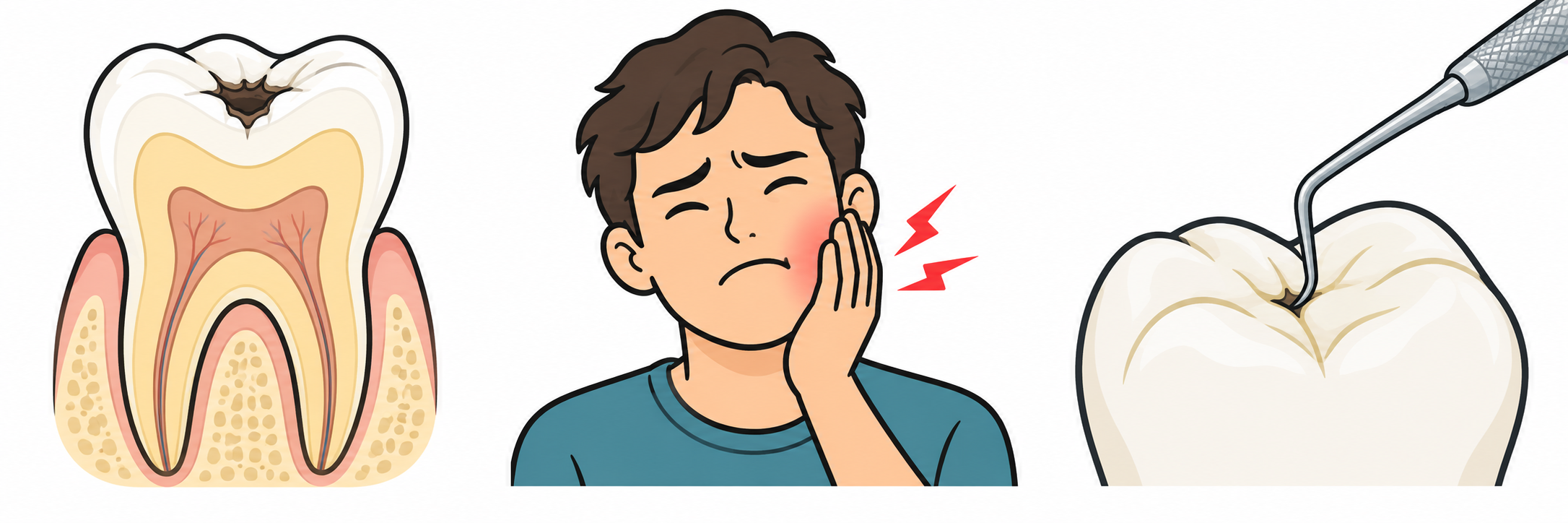
The hidden-value sums, filter/sum/normalize workflow, cavity network, and robot-room floor plan are original editable draw.io diagrams. Their source is joint-table-inference.drawio; the slides use PNG exports.
The toothache/cavity/probe-catch joint table follows Artificial Intelligence: A Modern Approach by Stuart Russell and Peter Norvig, fourth edition, Sections 12.3-12.5. The Bayesian-network preview follows Sections 13.1-13.2. The two-evidence and robot-sensor exercises are illustrative course examples, not clinical or measured sensor probabilities. See also the UC Berkeley CS 188 inference notes.
Lecture 23: Bayes Nets
The illustrated dental glossary reuses the same AI-generated cavity, toothache, and probe-catch cartoon as Lecture 22, with its generation prompt and provenance.
The prior-sampling trace, rejection counts, weighted counts, and Gibbs-state updates are original editable draw.io diagrams. Their source is bayes-network-sampling.drawio; the slides use PNG exports. The cavity-network diagram is reused from Lecture 22’s joint-table-inference.drawio.
The cavity/toothache/probe-catch model and sampling methods follow Artificial Intelligence: A Modern Approach by Stuart Russell and Peter Norvig, fourth edition, Sections 13.1-13.4. Probabilities, sample counts, and uniform draws are illustrative teaching examples, not clinical data or measured simulation results. See also the UC Berkeley CS 188 notes on Bayesian-network representation and approximate inference.
Lecture 24: Machine Learning
The training/prediction workflow, numerical neighbor-vote chart, PCA projection chart, robot feedback loop, and maze route are original editable draw.io figures. Their source is machine-learning-examples.drawio; the slides use PNG exports. Coordinates, feature-scale examples, evaluation counts, and robot rewards are constructed teaching examples.
The handwritten-digit figure is an unchanged saved image from the course’s KNN on MNIST notebook, using the MNIST handwritten-digit dataset distributed through Torchvision. It is not a newly run experiment. The public-domain OpenClipart brain/lightbulb icon is reused from Lecture 1.
The lecture follows the supplied Spring 2025 material and Artificial Intelligence: A Modern Approach by Stuart Russell and Peter Norvig, fourth edition, Sections 19.1-19.2. See also the scikit-learn documentation on nearest-neighbor methods and principal component analysis.
Lecture 25: Bias, Variance, and Overfitting
The campus courier cartoon and waiting-at-a-door cartoon were generated for this lecture using Codex’s built-in image generator. They illustrate the delivery-time example, not measured events or real people. The generation prompts and provenance are included with the assets.


The candidate delivery-time regression line, comparison of three polynomial fits, fixed-route bias/variance illustration, and the two error-versus-complexity charts are original editable data charts. Their source is regression-generalization.drawio, with data and formula notes; the slides use PNG exports. The campus delivery records, timing rule, and repeated-training predictions are invented teaching examples, not measured campus data. Delivery times use minutes; the later notebook is a separate random-feature experiment in its own output units. The polynomial fits illustrate a separate curved pattern and are calculated from the same seven constructed observations. The classical and double-descent curves are explicitly schematic, not measured notebook results or universal laws.
The lecture builds on the supplied Spring 2025 material and the course’s linear regression notebook. Technical references are the NumPy pseudoinverse documentation, scikit-learn’s bias-variance example, Belkin et al., Reconciling modern machine learning practice and the bias-variance trade-off, and Bartlett et al., Benign Overfitting in Linear Regression.
Lecture 26: Decision Trees and Random Forests
The tennis tree, three prediction-trace frames, Outlook split counts, delivery-time regression tree, bootstrap/feature-selection workflow, and forest leaf-output comparison are original editable draw.io diagrams. Their source is decision-forest-examples.drawio; the slides use PNG exports. The complete 14-day tennis table preserves the records supplied in the Spring 2025 Beamer lecture. The delivery values and forest leaf counts are invented teaching examples, not measured model results.
The tennis/weather cartoon and committee cartoon were generated for this lecture with Codex’s built-in image generator. They depict classroom concepts, not actual people or events. Their generation prompts and provenance are included with the assets.
Decision-tree concepts follow Artificial Intelligence: A Modern Approach, fourth edition, Section 19.3, and the supplied Spring 2025 material. Random-forest references are Breiman’s Random Forests (2001), the scikit-learn guide to decision trees, and its guide to random forests. The slides distinguish original majority voting from scikit-learn’s probability averaging.
Lecture 27: Practical PyTorch
The components/toolbox cartoon and tensor-check cartoon were generated using Codex’s built-in image generator. They illustrate software components and checking tensor shapes, not real people or reported experiments. The generation prompts and provenance are included.


The tensor-indexing, linear-layer-shape, and scalar-gradient figures are original editable draw.io diagrams, published as PNGs. Their source is pytorch-examples.drawio. The numerical arrays and derivatives are small constructed examples for learning syntax, not measured model results.
Technical references: PyTorch’s beginner quickstart, tensors, broadcasting, reshaping, datasets and data loaders, modules, linear layers, autograd, mean squared error, cross-entropy loss, gradient clearing, inference mode, checkpoint serialization, and reproducibility. Optional-tool references are TorchVision transforms v2, torch.compile, and automatic mixed precision. Working older interfaces such as no_grad() are not presented as deprecated.
Lecture 28: Deep Learning
The campus courier cartoon is reused unchanged from Lecture 25, where its generation prompts and provenance are recorded. The courier illustrates the delivery setting; the inputs, targets, initial parameters, derivatives, and updated predictions in this lecture are constructed teaching values, not measured delivery data.
The deep-layer overview and the five tiny-network views (parameter names, forward values, output gradients, hidden gradients, and inactive ReLU) are original editable draw.io diagrams, published as PNGs. Their source is neural-learning.drawio.
The lecture revises the supplied Spring 2025 Deep Learning Beamer source and follows Artificial Intelligence: A Modern Approach, U.S. fourth edition Section 21.1 / Global fourth edition Section 22.1. The Backpropagation notebook uses the same numeric example and unhalved mean-squared-error convention as the slides. Technical references are PyTorch’s autograd tutorial, MSELoss, ReLU, and SGD.
Lecture 29: Convolutional Neural Networks
The MNIST digit pixels reuse the unchanged saved notebook figure from Lecture 24. The slide layout shows only the digit strip, omitting its previous KNN prediction headings. These examples illustrate the input data, not new CNN predictions. See Lecture 24 for the original notebook and dataset source.
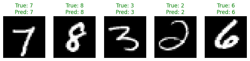
The numerical convolution setup, three animation frames, stride/padding illustration, channel diagram, ReLU map, max-pooling example, classifier head, and notebook architecture are original editable Draw.io diagrams. Their source is convolution.drawio; the slides use PNG exports. The convolution and pooling grids retain the constructed examples from the supplied Spring 2025 CNN Beamer source. They are teaching calculations, not learned filters or experimental model outputs.
The toy robot is unchanged public-domain OpenClipart artwork, reused from Lecture 1.

The shape walkthrough follows the existing single-digit CNN notebook. Technical references are PyTorch’s Conv2d, MaxPool2d, ReLU, Dropout, and CrossEntropyLoss, plus the official image-classifier tutorial.
Lecture 30: Reinforcement Learning
The agent/environment loop, delivery MDP, policy highlights, reward timing, model-based/model-free comparison, value-iteration frames, uncertain-move example, and policy-iteration figures are original editable Draw.io diagrams. Their source is mdp-planning.drawio; the slides use PNG exports. The delivery jobs, rewards, transition probabilities, and values are constructed teaching examples, not measurements or experimental results.
The toy robot is unchanged public-domain OpenClipart artwork, reused from Lecture 1.
The lecture manually revises the supplied Spring 2025 RL Beamer material, using a new numerical example consistently throughout. Background references are Artificial Intelligence: A Modern Approach, fourth edition, Sections 16.1-16.3 and 16.5, and the UC Berkeley CS 188 notes on Markov decision processes, value iteration, policy iteration, and reinforcement learning. Known-model planning and learning from experience are distinguished explicitly.
Lecture 31: Multi-Armed Bandits
The bandit cartoon is reused unchanged from the supplied Spring 2025 Beamer project. The original Beamer frame explicitly credits ChatGPT as its creator; the original generation prompt is unavailable. It is not presented as a CC0 asset.

The resource choices, feedback loop, observed-rating history, epsilon-greedy probabilities, two UCB score charts, sample-mean update, allocation comparison, and evaluation procedure are original course diagrams. Their editable Draw.io source contains nine pages, exported as PNGs for the slides. All reward histories, true means, and allocations are hypothetical teaching examples, not experiments with students or measured algorithm performance.
The lecture manually revises the supplied Spring 2025 bandit Beamer material. Background: Sutton and Barto, Reinforcement Learning: An Introduction, Chapter 2; Auer, Cesa-Bianchi, and Fischer, Finite-time Analysis of the Multiarmed Bandit Problem; and the authors’ Upper Confidence Bound exposition.
Lecture 32: Value-Based Model-Free RL
The public-domain toy robot is reused from Lecture 1. It represents a fictional learning agent, not a deployed robot system.
The observed transition, sample delivery episode, MC/TD update timing, behavior choice, SARSA target, Q-learning target, and return-horizon comparison are original course diagrams from this editable Draw.io source. The two-episode comparison and the DQN state-input and action-value network have separate editable Draw.io sources. The figures are exported as PNGs for the slides. All rewards and current estimates are constructed teaching examples. The new delivery service has unknown stochastic outcomes, illustrated by a failed pickup and varying delivery rewards. It reuses Lecture 30’s location names, not its known deterministic transition/reward model. The DQN diagram is an illustrative architecture with example predictions, not a trained model or empirical result.
The lecture manually revises the supplied Spring 2025 value-based RL Beamer material. Background references: Sutton and Barto, Reinforcement Learning: An Introduction, second edition, Chapters 5-7 and 12; the UC Berkeley CS 188 notes on reinforcement learning and model-free learning; David Silver’s Model-Free Prediction; and van Seijen et al., True Online Temporal-Difference Learning, for the distinction between conventional online traces and exact forward-view equivalence.
DQN and extensions: Volodymyr Mnih et al., Playing Atari with Deep Reinforcement Learning (2013) and Human-level control through deep reinforcement learning (2015); Hado van Hasselt, Arthur Guez, and David Silver, Deep Reinforcement Learning with Double Q-learning; Ziyu Wang et al., Dueling Network Architectures for Deep Reinforcement Learning; Tom Schaul et al., Prioritized Experience Replay; and Matteo Hessel et al., Rainbow: Combining Improvements in Deep Reinforcement Learning.
Lecture 33: Policy-Based Model-Free RL
The public-domain toy robot is reused from Lecture 1 as an illustrative learning agent.
The direct policy, sigmoid-probability bars, episode timeline, sampled-return-versus-baseline illustration, actor-critic loop, and critic transition are original course diagrams from this editable Draw.io source. The four sampled jobs have a separate editable Draw.io source. Figures are exported as PNGs for the slides. All rewards, parameter values, and numerical updates are constructed teaching calculations. The example uses a one-attempt variant of Lecture 32’s unknown stochastic delivery service: failed pickup cancels the current job, and job rewards can vary. Baselines and critic outputs are estimates, not known exact model values. No measured training performance is claimed.
The lecture manually revises the supplied Spring 2025 policy-based RL Beamer material. Background: Sutton and Barto, Reinforcement Learning: An Introduction, second edition, Chapter 13; Ronald J. Williams (1992), Simple statistical gradient-following algorithms for connectionist reinforcement learning; OpenAI Spinning Up’s Introduction to Policy Optimization; and the official PyTorch Tensor.detach documentation. The numerical walkthrough distinguishes expected advantage from sampled estimates, and uses explicit discount weights for its discounted starting-state objective.
Lecture 34: PPO, RLHF, DPO, and GRPO
The public-domain toy robot is reused from Lecture 1 as an illustrative agent.
The PPO round, old/candidate probability bars, positive and negative clipping curves, toy token policy, RLHF pipeline, preference pair, policy-role comparison, and response group are original course diagrams and calculated charts. Their editable Draw.io source contains nine pages, exported as PNGs for the slides. All probabilities, preferences, reward-model scores, and response groups are constructed teaching examples. They are not collected human feedback, outputs from a trained model, or measured training curves.
The DPO workflow is an additional original course diagram with its own editable Draw.io source. Its worked probability and loss values are constructed teaching examples, not measured model outputs.
The lecture manually revises the supplied PPO/GRPO Beamer material and adds an InstructGPT-style RLHF walkthrough and offline DPO. Primary references: John Schulman et al. (2017), PPO paper; Long Ouyang et al. (2022), InstructGPT/RLHF paper; Rafael Rafailov et al. (2023), DPO paper; and Zhihong Shao et al. (2024), DeepSeekMath/GRPO paper. The full paper titles and author credits appear at the methods’ first introductions in the deck. The official Spinning Up PPO explanation supports the clipping discussion. The curves distinguish positive and negative advantages and do not present clipping as a hard probability or KL bound.
Lecture 35: Generative Machine Learning
The binary-image dataset, sampling intervals, probability comparison, autoencoder, latent-code gap, normal-density chart, VAE paths, GAN training loop, diffusion paths, noising calculation, noise-prediction training, and coverage comparison are original editable course diagrams and data charts. Their Draw.io source contains twelve individually authored pages, exported as PNGs. The categorical probabilities, code locations, and numerical exercises are constructed teaching examples, not measured training results. The normal curve uses the stated mean and standard deviation.
The handwritten-digit image is reused unchanged from the course’s KNN on MNIST notebook, as in Lecture 24. It shows saved classification results on MNIST data distributed through Torchvision, not generated images or a new experiment.
The lecture develops the supplied Spring 2025 generative-ML material. Primary references: Kingma and Welling (2013), Auto-Encoding Variational Bayes; Goodfellow et al. (2014), Generative Adversarial Networks; Ho, Jain, and Abbeel (2020), Denoising Diffusion Probabilistic Models; and Heusel et al. (2017), the FID paper.
Lecture 36: Autoregressive Models
The generation cycle, completion probability, sampling intervals, teacher-forcing pairs, recurrent-state walkthrough, scalar update, output head, long dependency, LSTM memory path, GRU blend, raster ordering, causal mask, and three-image probability example are original editable course diagrams. Their Draw.io source contains thirteen individually authored pages, exported as PNGs. Text probabilities, logits, state and gate values, and the binary-image distribution are constructed examples, not trained-model results. The binary patterns and probabilities match Lecture 35.
The lecture develops the supplied Spring 2025 autoregressive-model material. State and gate conventions are checked against the official PyTorch documentation for RNN, LSTM, and GRU. The pixel ordering and masking discussion follows van den Oord, Kalchbrenner, and Kavukcuoglu (2016), Pixel Recurrent Neural Networks, which also introduces PixelCNN.
Lecture 37: Transformers
The context examples, generation pipeline, embedding lookup, query/key/value analogy, projection flow, worked attention calculation, column-normalization diagram, self/cross-attention comparison, training/generation comparison, quadratic-cost grids, and summary are original course illustrations. Their editable source is attention-worked-example.drawio; the slides use PNG exports of its fourteen individually authored pages.
The bank connections and train noticeboard are schematic illustrations, not measured model attention. The embedding coordinates, projected keys/values, and attention numbers are constructed examples; bar widths use the unrounded softmax weights. Architecture and attention concepts follow Ashish Vaswani et al. (2017), Attention Is All You Need. The row/column-layout comparison also refers to the official PyTorch attention documentation. These diagrams are not copied paper figures.
Lecture 38: Transformers Continued
The model pipeline, parallel heads, shifted targets, column-oriented causal mask, order example, position-frequency plot, rotary-vector example, residual update, normalization example, complete pre-LN block, vocabulary output, temperature bars, top-k filter, KV cache, perplexity example, image patches, diffusion pipeline, and summary are original course illustrations. Their editable source is transformer-components.drawio; the slides use PNG exports of its eighteen individually authored pages. Curves are sampled from the stated sine functions, and probability-bar widths use unrounded calculations. Numeric values and the small image pattern are constructed examples, not trained-model measurements or dataset images.
Architecture concepts develop the supplied Transformer Beamer/TikZ material and Vaswani et al. (2017), Attention Is All You Need. Further primary references are Jianlin Su et al. (2021), RoFormer: Enhanced Transformer with Rotary Position Embedding; Alexey Dosovitskiy et al. (2020/2021), An Image is Worth 16x16 Words: Transformers for Image Recognition at Scale; and William Peebles and Saining Xie (2022), Scalable Diffusion Models with Transformers.
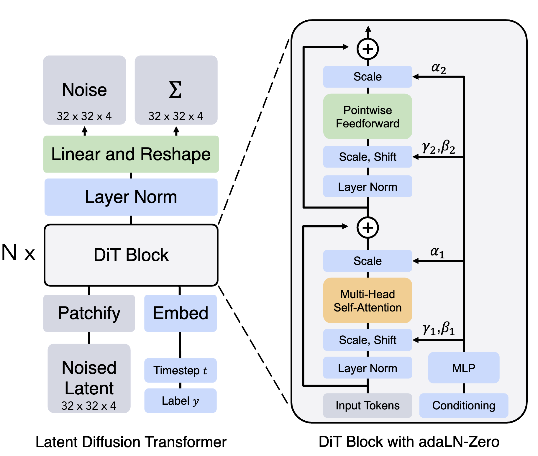
Normalization conventions are checked against the official PyTorch LayerNorm documentation. KV caching and perplexity are cross-checked with the official Hugging Face documentation on caching and perplexity. The supplied original DiT architecture figure, from Peebles and Xie’s paper, is retained as a supplementary reference; the revised slides use a simpler original pipeline diagram.
Lecture 39: Cutting-Edge AI Topics
The lecture-search system, adaptation choices, LoRA paths, quantized-base/adapters comparison, tool/skill/agent roles, skill package, LLM CLI workflow, MCP architecture, trust boundary, agent harness, example trace, evaluation pipeline, verification loop, search tests, and summary are original course illustrations. Their editable source is ai-system-components.drawio; the slides use PNG exports of its fifteen individually authored pages. Matrix values, parameter counts, app requirements, action traces, scores, and search-test data are constructed examples, not measurements of a trained model or product.
Adaptation and retrieval references: Edward J. Hu et al. (2021), LoRA: Low-Rank Adaptation of Large Language Models; Tim Dettmers et al. (2023), QLoRA: Efficient Finetuning of Quantized LLMs; Patrick Lewis et al. (2020), Retrieval-Augmented Generation for Knowledge-Intensive NLP Tasks.
Interface and workflow references: the official Agent Skills format, Codex CLI documentation, MCP architecture and tool-call examples, MCP security guidance, and EleutherAI Language Model Evaluation Harness. MCP snippets are explanatory tool-definition and call-parameter fragments, not complete protocol messages. The diagrams are original explanations of these concepts, not copied product screenshots.